Performing Fermi Edge Corrections
The most straightforward way to correct the Fermi edge, either due to monochromator miscalibration in a photon energy scan or due to using a straight slit on a hemispherical analyzer is just to broadcast an edge.
In the case of correcting for the slit shape, it may be helpful to further fit a model for the edge shape, like a quadratic, so that a smooth correction is applied across the detector.
Correcting monochromator miscalibration
[2]:
from arpes.io import example_data
from arpes.all import broadcast_model, AffineBroadenedFD

photon_energy = example_data.photon_energy
[3]:
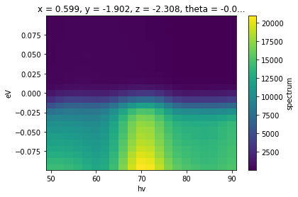
edge_data = photon_energy.sel(
    phi=slice(-0.28, -0.15), eV=slice(-0.1, 0.1)).sum("phi").spectrum
edge_data.T.plot()
[3]:
<matplotlib.collections.QuadMesh at 0x1e60065bfd0>
[4]:
import matplotlib.pyplot as plt
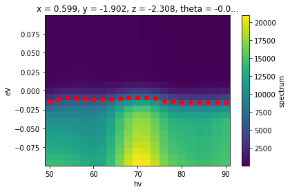
results = broadcast_model(AffineBroadenedFD, edge_data, "hv")
fig, ax = plt.subplots()
edge_data.T.plot(ax=ax)
ax.scatter(*results.F.p("fd_center").G.to_arrays(), color="red")
Running on multiprocessing pool... this may take a while the first time.
Deserializing...
Finished deserializing
[4]:
<matplotlib.collections.PathCollection at 0x1e601552a00>
Now, we can perform the shift to correct the edge.
[5]:
corrected_photon_energy = photon_energy.spectrum.G.shift_by(
    results.F.p("fd_center"), shift_axis="eV", shift_coords=True)
corrected_edge_data = corrected_photon_energy.sel(
    phi=slice(-0.28, -0.15), eV=slice(-0.1, 0.1)).sum("phi")

results_check = broadcast_model(AffineBroadenedFD, corrected_edge_data, "hv")

fig, ax = plt.subplots()
corrected_edge_data.T.plot(ax=ax)
ax.scatter(*results_check.F.p("fd_center").G.to_arrays(), color="red")
Running on multiprocessing pool... this may take a while the first time.
Deserializing...
Finished deserializing
[5]:
<matplotlib.collections.PathCollection at 0x1e6021bbe50>
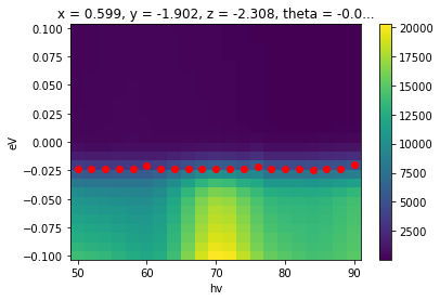
As we can see, the edge is now uniform across photon energy and correctly zero referenced.
A caveat to be aware of when shifting data is whether to make data adjustments only or to use coordinate adjustments as well. Coordinate adjustments (above: shift_coords=True) are useful when the shift is very large. If the coords are not allowed to compensate for some of the shift in that context, large portions of data will be shifted out of the array extent and be replaced by np.nan or 0.
However, if coordinates no longer agree between two pieces of data, we will not be able to perform array operations involving both of them, because of their incompatible coordinates.
The correct behavior is context dependent and requires you to consider what analysis you are trying to do.
Correcting the curved Fermi edges
Let’s now turn to an example addressing the uneven energy calibration arising from the use of a straight slit in ARPES data.
We will shortly turn to the question of momentum conversion, but we will want to have this issue corrected before converting. The correction we need to apply is a function of the detector angle phi, so it will not be a constant function of any momentum coordinate, in general.
First, let’s assess the data.
[6]:
from arpes.io import example_data
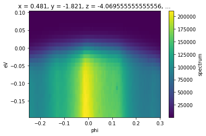
cut = example_data.map.sum("theta").spectrum
cut = cut.sel(eV=slice(-0.2, 0.1), phi=slice(-0.25, 0.3))
cut.S.plot()
Now, let’s fit edges to this data.
[7]:
from arpes.fits.utilities import broadcast_model
from arpes.fits.fit_models import AffineBroadenedFD, QuadraticModel
import matplotlib.pyplot as plt

results = broadcast_model(AffineBroadenedFD, cut, "phi")

results.F.plot_param("fd_center")
plt.gca().set_ylim([-0.05, 0.05])
Running on multiprocessing pool... this may take a while the first time.
Deserializing...
Finished deserializing
[7]:
(-0.05, 0.05)
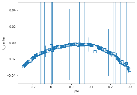
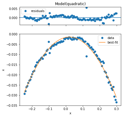
We could either refine these fits a little by setting some constraints, or we can make a smooth correction by fitting a quadratic to these edge locations.
[8]:
quad_mod = QuadraticModel().guess_fit(results.F.p("fd_center"))
quad_mod.plot()
[8]:
(<Figure size 432x432 with 2 Axes>, GridSpec(2, 1, height_ratios=[1, 4]))
Now, we can shift the data exactly like we did before. In order to get the shift amount to apply at each phi, we just evaluate our quadratic at these phi.
[9]:
fmap = example_data.map.spectrum
edge = quad_mod.eval(x=fmap.phi)

corrected_map = fmap.G.shift_by(edge, "eV")

fig, axes = plt.subplots(1, 2, figsize=(10, 5))
corrected_map.isel(theta=10).S.plot(ax=axes[0])
fmap.isel(theta=10).S.plot(ax=axes[1])

for ax in axes:
    ax.set_title("")
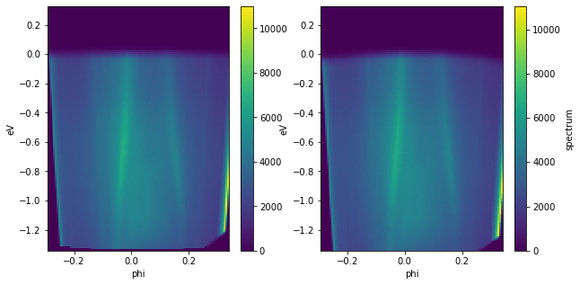
Much better. With this in order, we can now consider momentum conversion.
Exercises
Correct the Fermi edge on the Bi2Se3 cut data
example_data.cut. How does the presence of the dispersing surface state affect the range you should use?Perform a random shift of a Fermi edge using
.G.shift_by. Then, try to correct it. How close is your recovered correction to the original shift?