Non-ARPES Specific xarray Extensions
Whereas .S contains extensions specific to ARPES, general extensions to the xarray methods provided by PyARPES are found on the .G extension.
This extension is available on both xr.Dataset and xr.DataArray instances. For more detail, consult the docstrings and source for arpes.xarray_extensions.GenericAccessorTools.
Iteration
Iteration along one or more dimensions
iterate_axis allows iteration along one or more axes in the dataset. The produced value is a generator (you can think of this like a list) that contains pairs of coordinate values for the dimensions specified for iteration, and a cut of the data at those specific coordinates. As an example for ARPES, this allows you to iterate along either EDCs or MDCs by using .iterate_axis('phi') or .iterate_axis('eV') respectively.
Here is an example.
[2]:
# Set the random seed so that you get the same numbers
import numpy as np
np.random.seed(42)


import xarray as xr
import arpes.xarray_extensions # so .G is in scope

test_data = xr.DataArray(
    np.random.random((3,3)),
    coords={"X": [0, 1, 2], "Y": [-5, -4, -3]},
    dims=["X", "Y"]
)
test_data.values
[2]:
array([[0.37454012, 0.95071431, 0.73199394],
       [0.59865848, 0.15601864, 0.15599452],
       [0.05808361, 0.86617615, 0.60111501]])
[3]:
print("Constant X")
for coordinate, constant_x_cut in test_data.G.iterate_axis("X"):
    print(coordinate, constant_x_cut.values)

print("\nConstant Y")
for coordinate, constant_y_cut in test_data.G.iterate_axis("Y"):
    print(coordinate, constant_y_cut.values)
Constant X
{'X': 0} [0.37454012 0.95071431 0.73199394]
{'X': 1} [0.59865848 0.15601864 0.15599452]
{'X': 2} [0.05808361 0.86617615 0.60111501]

Constant Y
{'Y': -5} [0.37454012 0.59865848 0.05808361]
{'Y': -4} [0.95071431 0.15601864 0.86617615]
{'Y': -3} [0.73199394 0.15599452 0.60111501]
Iteration only across coordinates
iter_coords allows you to iterate across only the coordinates of a DataArray, without also iterating across the data values. This can be useful if you would like to transform the coordinates before selection, or would only like access to the coordinates.
[4]:
for coordinate in test_data.G.iter_coords():
    print(coordinate)
{'X': 0, 'Y': -5}
{'X': 0, 'Y': -4}
{'X': 0, 'Y': -3}
{'X': 1, 'Y': -5}
{'X': 1, 'Y': -4}
{'X': 1, 'Y': -3}
{'X': 2, 'Y': -5}
{'X': 2, 'Y': -4}
{'X': 2, 'Y': -3}
You can also iterate simultaneously over the coordinates and their indices in the data with enumerate_iter_coords.
[5]:
for index, coordinate in test_data.G.enumerate_iter_coords():
    print(index, coordinate)
(0, 0) {'X': 0, 'Y': -5}
(0, 1) {'X': 0, 'Y': -4}
(0, 2) {'X': 0, 'Y': -3}
(1, 0) {'X': 1, 'Y': -5}
(1, 1) {'X': 1, 'Y': -4}
(1, 2) {'X': 1, 'Y': -3}
(2, 0) {'X': 2, 'Y': -5}
(2, 1) {'X': 2, 'Y': -4}
(2, 2) {'X': 2, 'Y': -3}
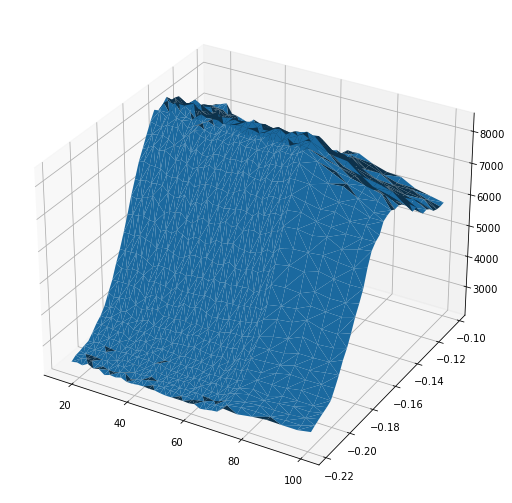
Raveling/Flattening
It is sometimes necessary to have access to the data in a flat format where each of the coordinates has the full size of the data. The most common usecase is in preparing an isosurface plot, but this functionality is also used internally in the coordinate conversion code.
The return value is a dictionary, with keys equal to all the dimension names, plus a special key “data” for the values of the array.
[6]:
from arpes.io import example_data
import matplotlib.pyplot as plt

data = example_data.temperature_dependence.spectrum.sel(
    eV=slice(-0.08, 0.05), phi=slice(-0.22, None)).sum("eV")

raveled = data.G.ravel()
fig = plt.figure(figsize=(9,9))
ax = fig.gca(projection="3d")

ax.plot_trisurf(
    raveled["temperature"], # use temperature as the X coordinates
    raveled["phi"],         # use phi as the Y coordinates
    data.values.T.ravel()   # use the intensity as the Z coordinate
)
[6]:
<mpl_toolkits.mplot3d.art3d.Poly3DCollection at 0x1e0b33d1130>
Coordinate manipulation
You can also get a flat representation of the coordinates and data of a one dimensional dataset using to_arrays. This is especially valuable since the result can be * splatted into an invocation of a scatter plot.
[7]:
one_dim = test_data.sum("X")
one_dim
[7]:
<xarray.DataArray (Y: 3)>
array([1.03128222, 1.97290909, 1.48910347])
Coordinates:
  * Y        (Y) int32 -5 -4 -3
- Y: 3
- 1.031 1.973 1.489
array([1.03128222, 1.97290909, 1.48910347])
- Y(Y)int32-5 -4 -3
array([-5, -4, -3])
[8]:
one_dim.G.to_arrays()
[8]:
(array([-5, -4, -3]), array([1.03128222, 1.97290909, 1.48910347]))
Functional Programming Primitives: filter and map
You can filter or conditionally remove some of a datasets contents. To do this over coordinates on a dataset according to a function/sieve which accepts the coordinate and data value, you can use filter_coord. The sieving function should accept two arguments, the coordinate and the cut at that coordinate respectively. You can specify which coordinate or coordinates are iterated across when filtering using the coordinate_name paramter.
As a simple, example, we can remove all the odd valued coordinates along Y:
[9]:
test_data.G.filter_coord("Y", lambda y, _: y % 2 == 0)
[9]:
<xarray.DataArray (X: 3, Y: 1)>
array([[0.95071431],
       [0.15601864],
       [0.86617615]])
Coordinates:
  * X        (X) int32 0 1 2
* Y (Y) int32 -4- X: 3
- Y: 1
- 0.9507 0.156 0.8662
array([[0.95071431], [0.15601864], [0.86617615]]) - X(X)int320 1 2
array([0, 1, 2])
- Y(Y)int32-4
array([-4])
Functional programming can also be used to modify data. With map we can apply a function onto a DataArray’s values. You can use this to add one to all of the elements:
[10]:
test_data.G.map(lambda v: v + 1)
[10]:
<xarray.DataArray (X: 3, Y: 3)>
array([[1.37454012, 1.95071431, 1.73199394],
       [1.59865848, 1.15601864, 1.15599452],
       [1.05808361, 1.86617615, 1.60111501]])
Coordinates:
  * X        (X) int32 0 1 2
* Y (Y) int32 -5 -4 -3- X: 3
- Y: 3
- 1.375 1.951 1.732 1.599 1.156 1.156 1.058 1.866 1.601
array([[1.37454012, 1.95071431, 1.73199394], [1.59865848, 1.15601864, 1.15599452], [1.05808361, 1.86617615, 1.60111501]]) - X(X)int320 1 2
array([0, 1, 2])
- Y(Y)int32-5 -4 -3
array([-5, -4, -3])
Additionally, we can simultaneously iterate and apply a function onto a specified dimension of the data with map_axes. Here we can use this to ensure that the rows along Y have unit norm.
[11]:
test_data.G.map_axes("Y", lambda v, c: v / np.linalg.norm(v))
[11]:
<xarray.DataArray (X: 3, Y: 3)>
array([[0.52859931, 0.73382829, 0.76253974],
       [0.84490405, 0.12042618, 0.16250411],
       [0.08197508, 0.66857578, 0.62619929]])
Coordinates:
  * X        (X) int32 0 1 2
* Y (Y) int32 -5 -4 -3- X: 3
- Y: 3
- 0.5286 0.7338 0.7625 0.8449 0.1204 0.1625 0.08198 0.6686 0.6262
array([[0.52859931, 0.73382829, 0.76253974], [0.84490405, 0.12042618, 0.16250411], [0.08197508, 0.66857578, 0.62619929]]) - X(X)int320 1 2
array([0, 1, 2])
- Y(Y)int32-5 -4 -3
array([-5, -4, -3])
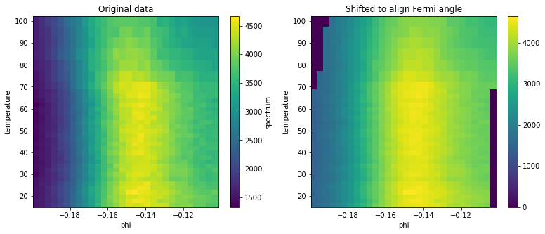
Shifting
Suppose you have a bundle of spaghetti in your hand with varying lengths. You might want to align them so that they all meet in a flat plane at the tops of the strands. In general, you will have to shift each a different amount depending on the length of each strand, and its initial position in your hand.
A similar problem presents itself in multidimensional data. You might want to shift 1D or 2D “strands” of data by differing amounts along an axis. One practical use case in ARPES is to align the chemical potential to take into account the spectrometer calibration and shape of the spectrometer entrance slit. Using the curve fitting data we explored in the previous section, we can align the data as a function of the temperature so that all the Fermi momenta are at the same index:
[12]:
# first, get the same cut and fermi angles/momenta from the previous page
# this is reproduced for clarity and so you can run the whole notebook
# please feel free to skip...

from arpes.fits.utilities import broadcast_model
from arpes.fits.fit_models import LorentzianModel, AffineBackgroundModel

temp_dep = example_data.temperature_dependence
near_ef = temp_dep.sel(
    eV=slice(-0.05, 0.05),
    phi=slice(-0.2, None)
).sum("eV").spectrum

phis = broadcast_model(
    [AffineBackgroundModel, LorentzianModel], near_ef, "temperature",
).F.p("b_center")

# ...to here
fig, ax = plt.subplots(1, 2, figsize=(13, 5))
near_ef.S.plot(ax=ax[0])
near_ef.G.shift_by(phis - phis.mean(), shift_axis="phi").S.plot(ax=ax[1])

ax[0].set_title("Original data")
ax[1].set_title("Shifted to align Fermi angle")
Running on multiprocessing pool... this may take a while the first time.
Deserializing...
Finished deserializing
[12]:
Text(0.5, 1.0, 'Shifted to align Fermi angle')