Tutorial data in PyARPES

As of v3, PyARPES includes four samples of data you can use to start learning how to conduct an analysis. Realism is important in tutorials, so PyARPES includes common types of data you’ll produce during experiments at synchrotrons.

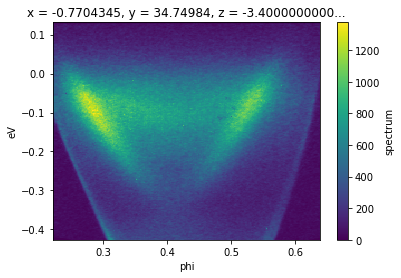
1. cut: an Energy and momentum “cut” at laser-UV photon energies across the gamma point of Bi_2Se_3.

2. map: an angle-angle “map” at soft X-ray photon energies of a metal

3. photon_energy: an angle-photon energy scan at soft X-ray energies from a metal

4. nano_xps: a scanning XPS image at soft X-ray energies from WS2

5. temperature_dependence: a temperature resolved ARPES cut at soft X-ray energies

All samples are moderately binned to respect user’s bandwidth and repository hosting constraints.

If you would like to contribute a piece of sample data or want to request a particular type of data be available in future release, please let the maintainers know.

Demo analyses use only these included data samples. This means you can cut-and-paste or download analysis notebooks to try them on your computer.

Each analysis notebooks has a few learning exercises in a section at the end.

Accessing tutorial data

To access tutorial data here or in your notebooks, you just import example_data from arpes.io.

from arpes.io import example_data

bi2se3_cut = example_data.cut # <- here, take `cut` above
                              # any of `map`, `photon_energy`,
                              # `nano_xps`, or
                              # `temperature_dependence` will work

# the last line of a Jupyter cell is "printed", printing a
# piece of ARPES data gives a rich representation
bi2se3_cut

<xarray.Dataset>
Dimensions:   (eV: 240, phi: 240)
Coordinates:
  * phi       (phi) float64 0.2217 0.2234 0.2251 0.2269 ... 0.6353 0.637 0.6388
  * eV        (eV) float64 -0.4256 -0.4233 -0.4209 ... 0.1256 0.1279 0.1302
    x         float64 -0.7704
    y         float64 34.75
    z         float64 -3.4e-05
    theta     float64 0.0
    beta      float64 0.0
    chi       float64 -0.1091
    hv        float64 5.93
    alpha     int32 0
    psi       int32 0
Data variables:
    time      float64 0.0
    spectrum  (phi, eV) int32 1 2 0 6 45 72 35 37 64 ... 62 76 82 95 84 74 72 42
Attributes: (12/97)
    file:                      c:\users\chsta\documents\github\arpes\arpes\ex...
    location:                  ALG-MC
    BITPIX:                    8
    NAXIS:                     0
    START_T:                   2/3/2016 1:45:34 PM
    START_TS:                  3537380734.727
    ...                        ...
    perpendicular_deflectors:  False
    analyzer_radius:           150
    analyzer_type:             hemispherical
    mcp_voltage:               None
    probe_linewidth:           0.015
    chi_offset:                -0.10909301748228785

# just transpose to a more natural axis order with `.T` and plot
bi2se3_cut.spectrum.T.plot()

<matplotlib.collections.QuadMesh at 0x256a31015b0>

Exercises

The PyARPES data model

1. Look through the HTML representation of example_data.cut. How do the coordinates correspond to the PyARPES spectral representation?

2. Skim the attrs section from the HTML representation of example_data.cut

3. PyARPES relies on xarray to provide it’s “Wave” representation, have a look at the xarray documentation to learn how to manipulate them.