Brillouin Zones

Some support for calculating and plotting Brillouin zones in PyARPES is included via ASE, the Atomic Simulation Environment. You will need to install ase as an optional dependency, for instance via pip, in order to use functions associated with plotting Brillouin zones in PyARPES.

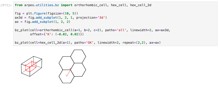
Importantly, PyARPES wraps two functions bz2d_plot and bz3d_plot from ase.dft.bz for displaying Brillouin zones in 2 and 3 dimensions. These functions include additional functionality to plot additional zones (the repeat= parameter), to change rendering settings, and to provide a consistent interface with the rest of the plotting utilities in PyARPES.

Plotting zones in 2D and 3D

Drawing Brillouin zones in 2D and 3D

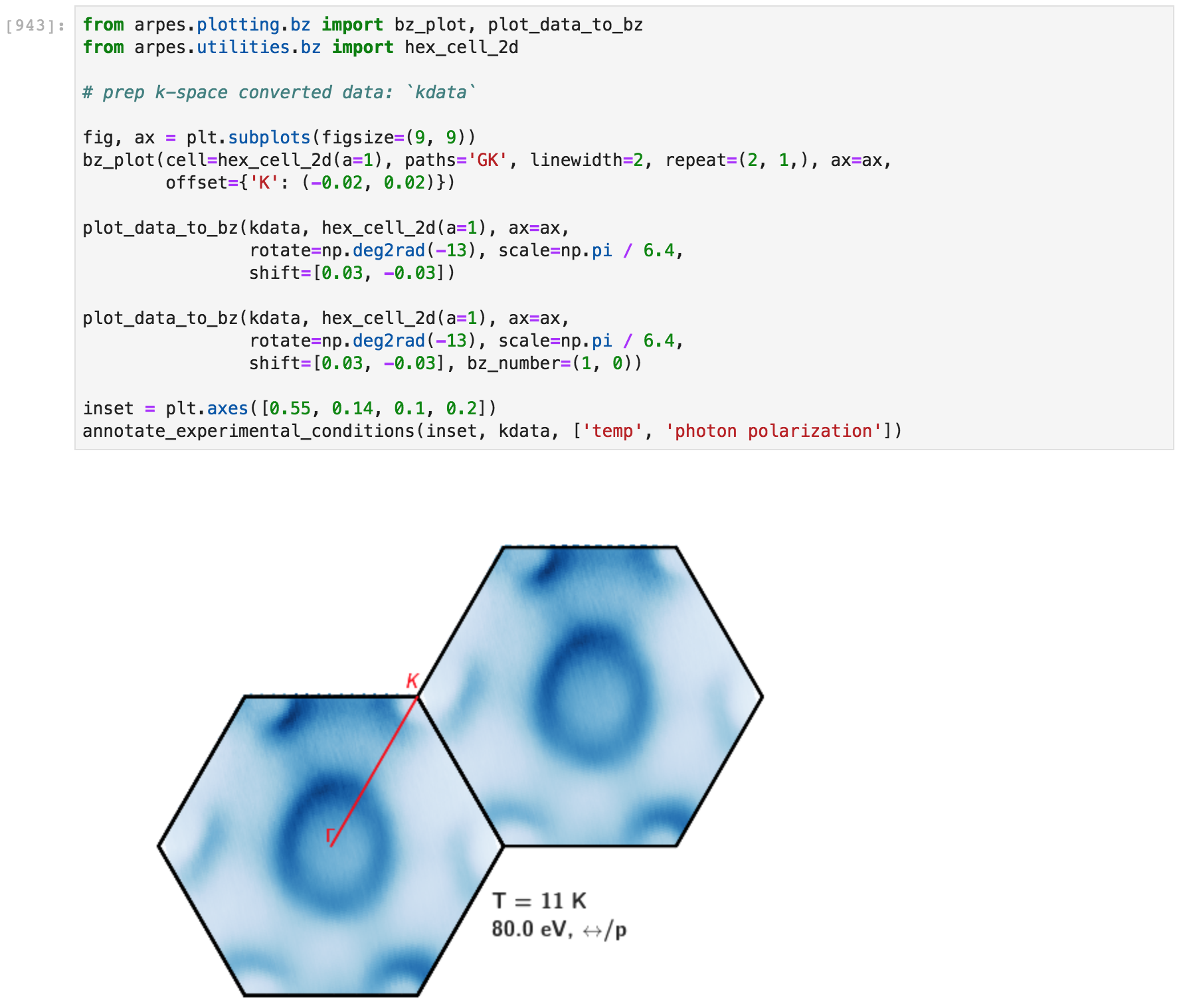
Plotting ARPES data onto 2D zones

As an example, we can plot low temperature ARPES data of 2H-NbS2 onto the appropriate hexagonal Brillouin zone. The data must first be converted to momentum space, stored here as kdata.

Additional Brillouin zones can be addressed with the bz_numberparameter.

Plotting ARPES data onto Brillouin zones

Note: PyARPES does not currently support plotting data onto 3D Brillouin zones, but we anticipate that this will be supported in future releases.

Plotting cut locations onto 3D zones

Frequently it is beneficial to indicate the schematic location of a 2D arpes cut onto the 3D zone, neglecting the dispersion of kz in the case of in-plane momentum maps.

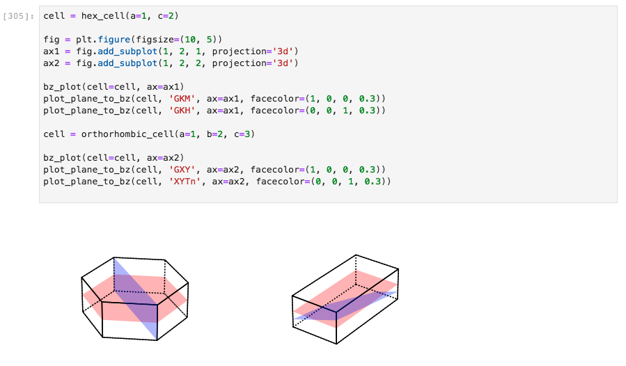
Plotting cuts through zones

Plotting paths through 2D and 3D zones

Paths through zones can also be plotted. PyARPES supports paths defined by high symmetry points (G, Y, L, etc.), as well as the negatives of these points (as vectors relative to zone center), for instance Gn. Furthermore, you can access symmetry points in second and higher zones, with K(1, 0, 0) in 3D or with G(0, 1) in two dimensions, as examples.

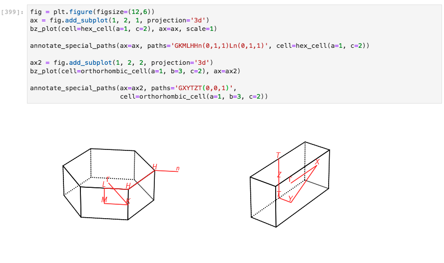
Paths through Brillouin zones